1. SUM
Syntax :
=SUM(number1, [number2], [number3], ...)
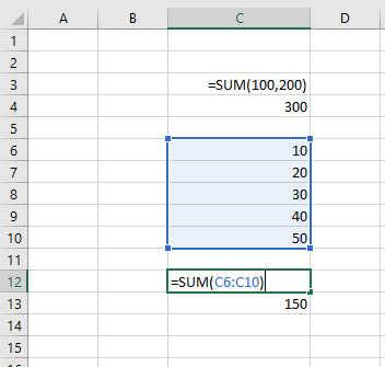
Example : =SUM(100, 200) => 300
Note: Excel also provides selecting multiple or range of cells if the number set is large as shown in the image below.
 |
|---|
| SUM |
2. AVERAGE
Syntax :
=AVERAGE(number1, [number2], [number3], ...)
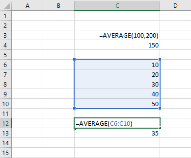
Example : =AVERAGE(100, 200) => 150
Note: Excel also provides selecting multiple or range of cells if the number set is large as shown in the image below.
 |
|---|
| AVERAGE |
3. SUMIF
Syntax :
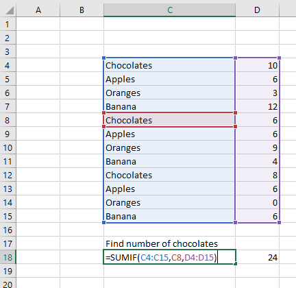
=SUMIF(range, criteria, [sum_range])
Example : Find number of chocolates from the list -
 |
|---|
| SUMIF |
4. COUNT
Syntax :
=COUNT(value1, [value2], [value3], ...)
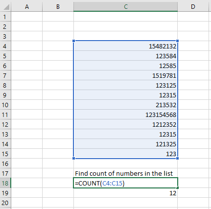
The COUNT function counts the number of cells that contain numbers, and counts numbers within the list of arguments.
Empty cells, logical values, text, or error values in the array or reference are not counted.
Example : Find count of numbers in the list -
 |
|---|
| COUNT |
5. COUNTA
Syntax :
=COUNTA(value1, [value2], [value3], ...)
-
The COUNTA function counts the number of cells that are not empty in a range.
-
The COUNTA function counts cells containing any type of information, including error values and empty text (“”).
For example, if the range contains a formula that returns an empty string, the COUNTA function counts that value.
- The COUNTA function does not count empty cells.
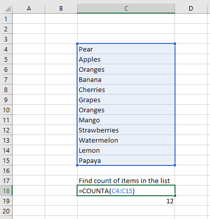
Example : Find count of items in the list -
 |
|---|
| COUNTA |
Additional Notes :
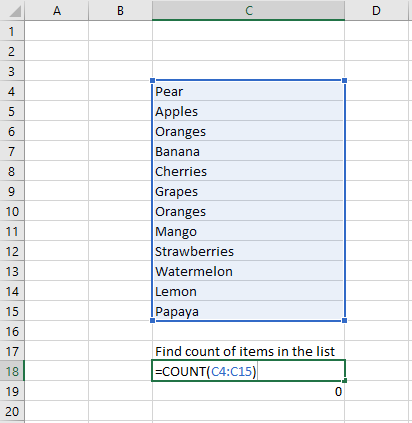
- If you use COUNT to find the count of items in the list, it gives ZERO
 |
|---|
| COUNT vs COUNTA |
6. COUNTIF
To count the number of times a particular text appears in a list.
Syntax :
=COUNTIF(range, criteria)
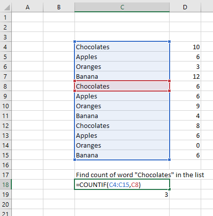
Example : Find count of word “Chocolates” in the list
 |
|---|
| COUNTIF |
7. CONCATENATE
To join two or more text strings into one string.
Syntax :
=CONCATENATE(text1, [text2], [text3], ...)
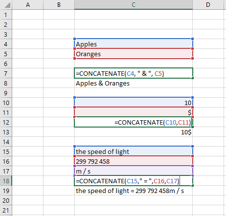
Example :
 |
|---|
| CONCATENATE |
8. IF
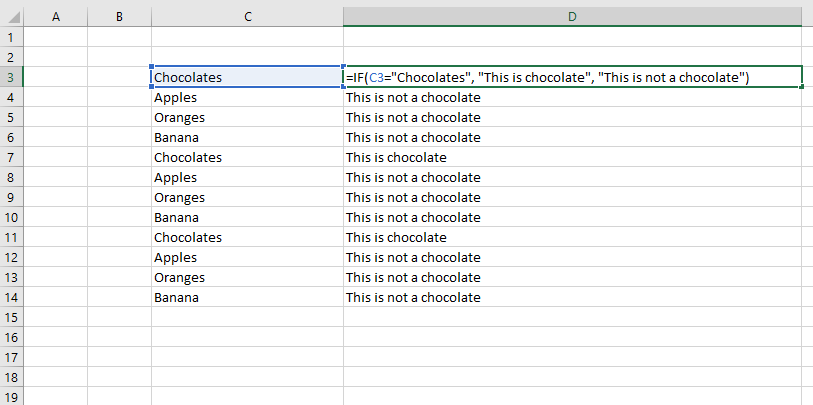
It allows you to make logical comparisons between a value and what you expect.
Syntax :
=IF(logical_test, value_if_true, [value_if_false])
 |
|---|
| IF |
9. VLOOKUP
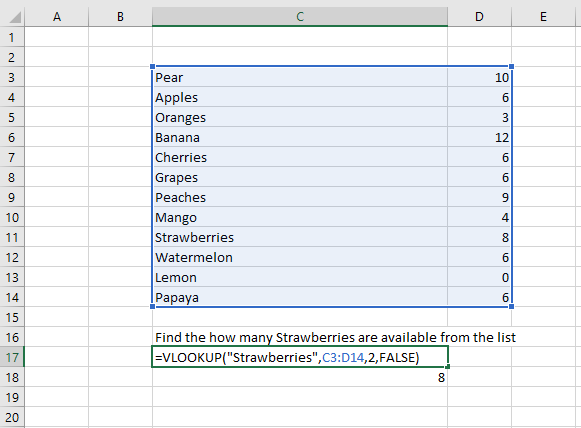
Use VLOOKUP when you need to find things in a table or a range by row.
Syntax :
=VLOOKUP (lookup_value, table_array, col_index_num, [range_lookup])
Example : Find the how many Strawberries are available from the list
 |
|---|
| VLOOKUP |
10. Conditional Formatting
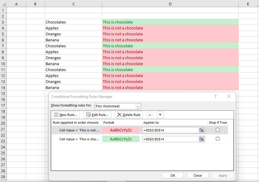
Conditional formatting in Excel enables you to highlight cells with a certain color, depending on the cell’s value.
For Example, if the text says “This is chocolate” it should be GREEN else it should be RED.
 |
|---|
| Conditional Formatting |
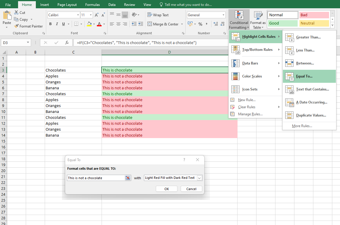
On the Home tab, in the Styles group, click Conditional Formatting > Click Highlight Cells Rules > Equal To…
Create two rules, one for text “This is chocolate” which should be “Green fill with Dark Green Text” & another for “This is not a chocolate” for “Light Red fill with Dark Red Text”.
 |
|---|
| Apply Conditional Formatting |